Neural Networks — Quick Notes to Get Up to Speed
The idea behind this write-up is to gather basic information and put it in the form of quick notes — so anyone reading it, including myself, can understand things without spending too much time looking through multiple places. There is a lot of content out there on AI, but most of it either goes too deep into theory or assumes you already know the basics. This is an attempt to bridge that gap.
Coming from a network background and working in AI ops, knowing these basics is something I need too. AI is no longer just a research topic — it is part of the infrastructure, the tooling, and the day-to-day decisions. Having a clear picture of how these systems work, even at a basic level, makes a real difference.
This is what I know so far, and I will keep enhancing it over time. Instead of going deep into theory, it focuses on the basic ideas — just enough to understand what is happening and why.
Neural Networks
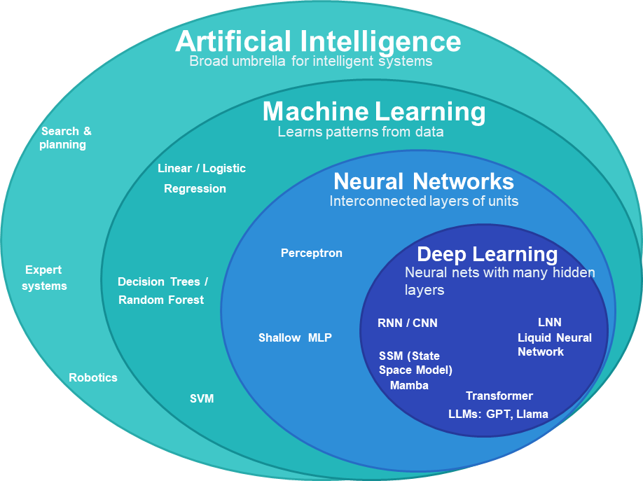
AI is any system that can do things that normally require human intelligence — understanding language, recognising images, making decisions.
Machine Learning is one way to build AI. Instead of writing explicit rules, you feed the system data and let it figure out the rules on its own.
Traditional programming: Rules + Data → Answer
Machine learning: Data + Answers → Rules
Neural Networks are one type of ML. Loosely inspired by how neurons in the brain work — each node takes inputs, multiplies each by a weight (importance), adds a bias, then passes the result through an activation function:
- w = weight — how much does this input matter?
- b = bias — how easily does this neuron fire?
- f = activation function — adds non-linearity so the network can learn complex patterns
Deep Learning is just neural networks with many hidden layers. More layers → more abstract representations the model can learn.
Not all Neural Networks are Deep Learning, but all Deep Learning is Neural Networks.
Types of Neural Networks
Different architectures suit different types of data:
Feed-Forward Network (FNN) — simplest. Input → hidden layers → output, one direction, no memory. Used for classification and tabular data.
CNN (Convolutional Neural Network) — built for images. Scans local patches, builds up from edges → shapes → objects. Examples: Google Photos (image search and auto-tagging), Apple Face ID, Tesla Autopilot vision system, Instagram/Snapchat filters.
RNN (Recurrent Neural Network) — built for sequences (text, speech, time series). Remembers previous inputs while processing the next. In “The movie was not good”, it needs “not” in memory when it reaches “good”. Problem: memory fades over long sequences.
State Space Models (SSM) — also for sequences, but handle long contexts more efficiently than RNNs. Compress past information into a compact internal state rather than carrying every token. Examples: S4, Mamba.
Transformers — look at the entire sequence at once, using attention to decide which parts relate to which. No word-by-word processing. This makes them faster to train and much better at long-range relationships. Most modern LLMs (GPT, Llama, Gemini, Claude) are transformer-based.
GPU and the Hardware Behind AI
Neural networks — especially large ones — need to do an enormous number of matrix multiplications, additions, and activation functions. A CPU can do this, but slowly. A GPU is built for exactly this kind of work.
CPU vs GPU — the simple version:
- A CPU has a small number of powerful cores. Great at complex logic, branching, sequential tasks — like a master chef who can cook anything but handles one thing at a time.
- A GPU has thousands of smaller cores all running in parallel — like a McDonald’s kitchen where every worker repeats the same operation at high speed.
AI training is basically the same calculation repeated millions of times on huge amounts of data. That’s a GPU’s sweet spot.
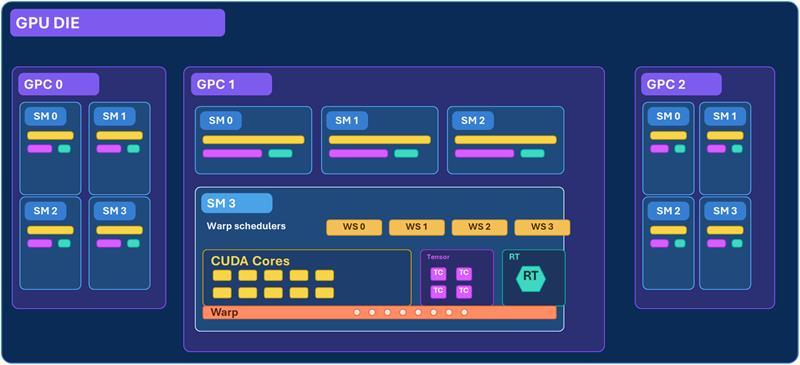
Inside a GPU
A GPU is organized into Streaming Multiprocessors (SMs) — each one is a mini compute unit containing:
- CUDA cores — general-purpose arithmetic (integer, float, vector math). Used for tokenization, embeddings, positional encoding, softmax, layer norm, residual connections.
- Tensor cores — specialized for matrix multiplication. Much faster than CUDA cores for neural network ops. Used for attention calculations, feed-forward layers, backpropagation. Run in lower precision: FP16, BF16 (training) or INT8 (inference).
- Warp schedulers — decide which group of threads runs next.
Threads and Warps:
GPU threads are grouped in warps of 32. All 32 threads execute the same instruction simultaneously, each on a different piece of data — this is called SIMT (Single Instruction, Multiple Threads). If threads in the same warp need to follow different code paths — branching, meaning if/else conditions where some threads go one way and others go another — they split and some sit idle. This is called warp divergence. GPUs hate branching; they love repetition.
FMA (Fused Multiply-Add):
The core operation a GPU is optimized for:
One instruction. This is exactly what a neuron computes: wx + b.
CPU vs GPU — Another Way to Think About It
| CPU | GPU | |
|---|---|---|
| Analogy | Jumbo jet | Cargo ship |
| Cores | Few, powerful | Thousands, smaller |
| Best at | Complex logic, low latency | Massive parallel computation |
| AI role | Control, preprocessing | Training and inference |
LLM Memory (VRAM)
When a model runs on a GPU, all its parameters must fit in VRAM. A rough rule:
| Precision | Bytes/param | 7B model | 70B model |
|---|---|---|---|
| FP32 | 4 | ~28 GB | ~280 GB |
| FP16 / BF16 | 2 | ~14 GB | ~140 GB |
| INT8 | 1 | ~7 GB | ~70 GB |
| 4-bit | 0.5 | ~3.5 GB | ~35 GB |
Actual usage is higher — the GPU also needs memory for the KV cache, activations, temporary tensors, and optimizer states during training. Large models are often split across multiple GPUs.
Quantization — store weights in lower precision (INT8, 4-bit) to cut VRAM and speed up inference. Tradeoff: too aggressive and accuracy drops.
Distillation — train a small student model to mimic a large teacher model. The student learns from the teacher’s outputs, not raw data. Result: a smaller, faster model that retains most of the capability.
Fine-tuning — take a pre-trained model and continue training it on a smaller, task-specific dataset. The weights already learned during pre-training are adjusted to make the model better at a specific task or domain. For example, taking a general-purpose LLM and fine-tuning it on medical records to make it better at clinical language. Much cheaper than training from scratch since the model already understands language — you are just steering it.
Other Chips Worth Knowing
APU (Accelerated Processing Unit) — CPU and GPU combined on one chip (common in laptops and phones).
FPGA (Field Programmable Gate Array) — reconfigurable hardware. Used in networking, telecom, and some AI acceleration.
NPU (Neural Processing Unit) — chip designed specifically for AI. Found in modern phones, PCs, cars, and IoT devices. Runs AI models efficiently at low power — handles on-device inference without needing a cloud GPU.
LLM Training
Large Language Models (LLMs) are not trained in a single step. The process happens in stages, where each stage builds on top of the previous one.
At a high level, training starts with pre-training on massive amounts of unlabeled data, where the model learns language patterns by predicting the next token. This gives us a base model that understands grammar, structure, and general knowledge.
This is followed by post-training, where the model is refined using human guidance. First, supervised fine-tuning (SFT) teaches the model how to respond properly using labeled examples. Then, a reward model is trained based on human feedback to understand which responses are better.
Finally, reinforcement learning is applied to optimize the model using this reward signal, aligning it with human preferences.
This multi-stage pipeline is what makes modern LLMs both powerful and usable in real-world applications.
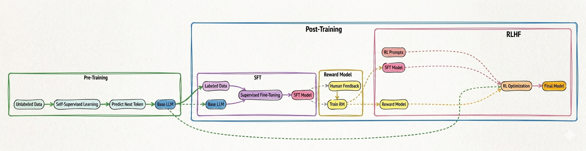 Figure: Overview of LLM training — pre-training builds language understanding, while post-training (SFT and RLHF) refines the model using human feedback and reward-based optimization.
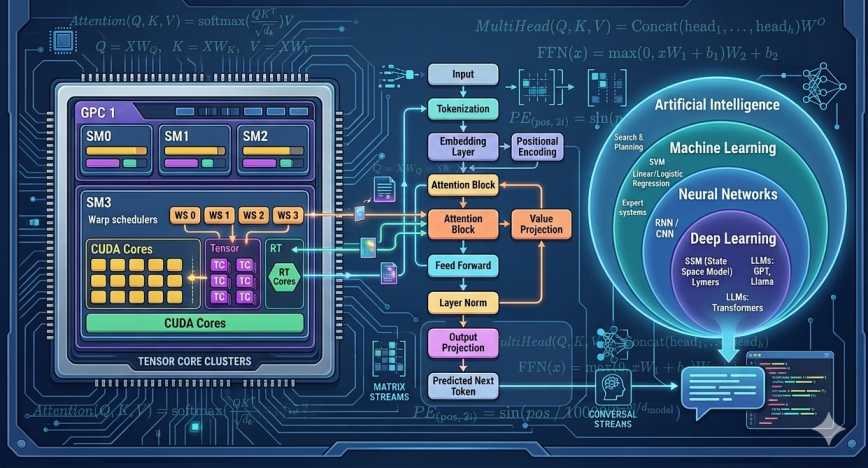
Pre-Training — Inside the Transformer
Now that we understand the overall training pipeline, let’s zoom into the pre-training stage and see how the transformer actually works internally.
Here’s the full transformer pipeline, step by step:
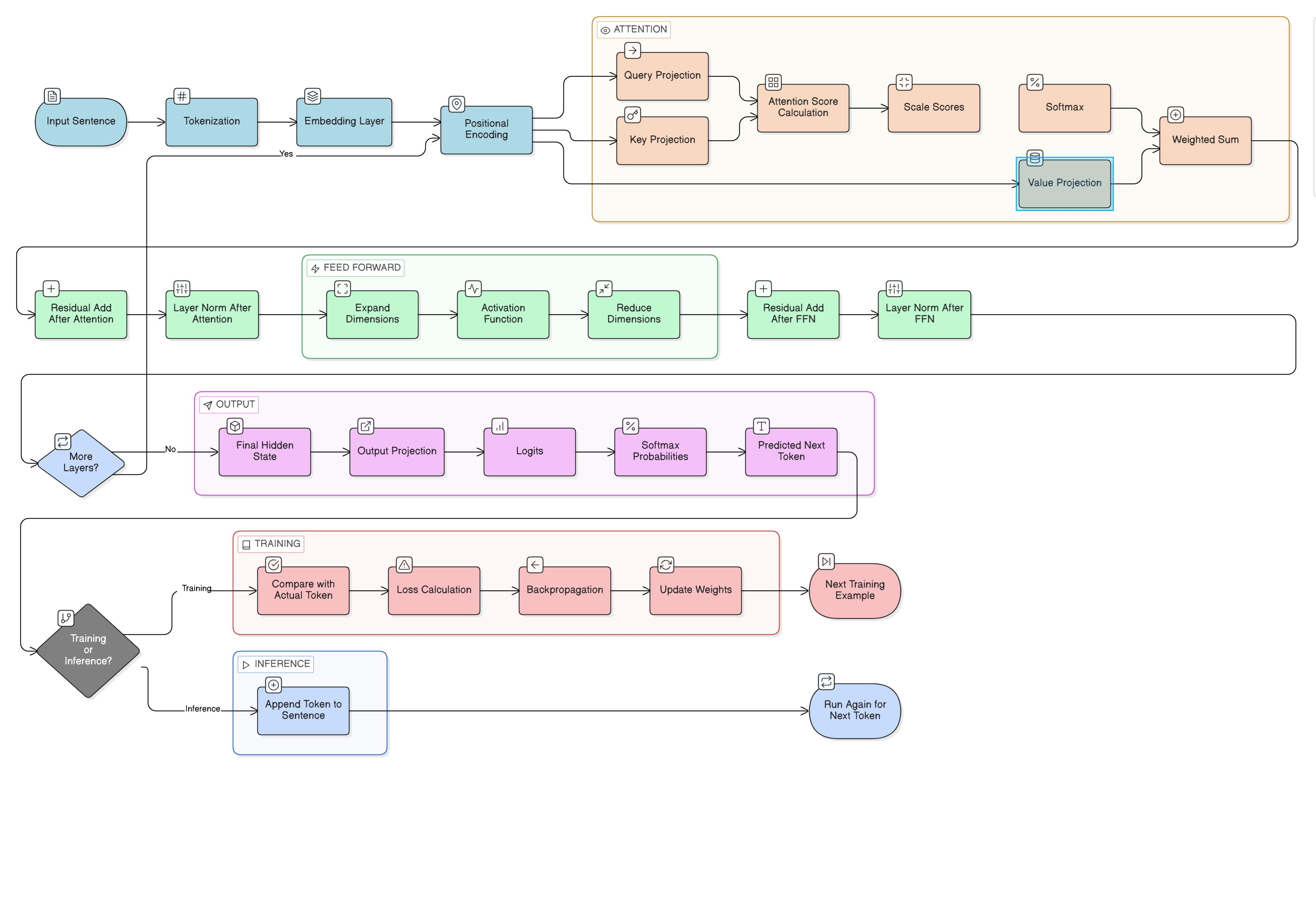 Figure: The complete transformer pipeline — from raw text to predicted next token, covering tokenization, embedding, attention, feed-forward layers, and the training/inference branches.
Part 1 — Tokenization: Breaking Language into Pieces
The first thing a transformer does is convert raw text into something it can actually work with numerically. That process is called tokenization.
Imagine a sentence:
“The cat sat on the mat”
A transformer cannot directly understand words the way humans do. It first converts text into smaller pieces called tokens. These tokens are not always whole words. The tokenizer breaks language into subword units — pieces that strike a balance between vocabulary size and coverage.
For example:
"playing"may become:"play""ing"
"unhappiness"may become:"un""happy""ness"
This approach is powerful because the model can reuse known pieces to understand words it has never seen before. For example, even if the model never encountered "cyberwarfare" during training, it may already know:
"cyber""war""fare"
Once the sentence is split into tokens, each token is assigned an integer ID from the vocabulary.
Example — Tokenizing “The cat sat”:
| Token | ID |
|---|---|
| The | 104 |
| cat | 587 |
| sat | 982 |
At this point, the model still does not know meaning. It only has integer IDs.
Part 2 — Embedding: Converting IDs into Meaningful Vectors
A raw integer ID carries no semantic weight. The number 587 does not tell the model anything about cats. So the next step converts each token ID into a vector of floating-point numbers — a representation that can actually encode meaning.
Instead of:
cat = 587
It becomes something like:
This vector can have hundreds or thousands of dimensions. The embedding space is learned during training — it is not hand-crafted. Concepts that are semantically similar end up with similar vector patterns.
For example, after training:
"cat","dog","lion"— may end up clustered close together in the embedding space"car","engine","truck"— may form a separate cluster
The embedding matrix is trainable. Initially it starts random, but after training on vast amounts of text, similar concepts acquire similar vector patterns.
The input now becomes a matrix where:
- Rows = tokens
- Columns = embedding dimensions
So if you have 10 tokens and embedding dimension = 768, the input matrix becomes:
10 × 768
Example — Embedding “The cat sat” with dimension = 4:
| Token | Embedding Vector | Shape |
|---|---|---|
| The | \(\left[\,{\color{#1A5276}{0.2}},\ {\color{#1A5276}{0.8}},\ {\color{#1A5276}{-0.1}},\ {\color{#1A5276}{0.5}}\,\right]\) | 1 × 4 |
| cat | \(\left[\,{\color{#1A5276}{0.9}},\ {\color{#1A5276}{-0.3}},\ {\color{#1A5276}{0.7}},\ {\color{#1A5276}{0.1}}\,\right]\) | 1 × 4 |
| sat | \(\left[\,{\color{#1A5276}{0.4}},\ {\color{#1A5276}{0.6}},\ {\color{#1A5276}{-0.2}},\ {\color{#1A5276}{0.9}}\,\right]\) | 1 × 4 |
When we stack all token vectors together, we get the embedding matrix X:
\[X = \begin{bmatrix} 0.2 & 0.8 & -0.1 & 0.5 \\ 0.9 & -0.3 & 0.7 & 0.1 \\ 0.4 & 0.6 & -0.2 & 0.9 \end{bmatrix}\]Shape: 3 × 4 — 3 rows (tokens) × 4 columns (embedding dimension)
Part 3 — Positional Encoding: Giving Order to the Tokens
Here is a subtle but critical problem: embeddings alone have no sense of order.
Consider:
“Dog bites man” “Man bites dog”
These two sentences contain the exact same words — and therefore the exact same token embeddings — but carry completely different meanings. Without positional information, the model cannot distinguish them.
To fix this, a positional encoding vector is added to each token’s embedding. This positional vector tells the model:
- this token is first
- this token is second
- this token is third
The position vector is simply added to the embedding vector element-wise. After this step, every token contains two kinds of information blended together:
- Meaning information (from the embedding)
- Position information (from the positional encoding)
This combined matrix becomes the input to the first transformer layer.
Example — Positional vectors for “The cat sat”:
| Position | Position Vector |
|---|---|
| 1 | \(\left[\,{\color{#1E6B4A}{0.1}},\ {\color{#1E6B4A}{0.0}},\ {\color{#1E6B4A}{0.1}},\ {\color{#1E6B4A}{0.0}}\,\right]\) |
| 2 | \(\left[\,{\color{#1E6B4A}{0.0}},\ {\color{#1E6B4A}{0.1}},\ {\color{#1E6B4A}{0.0}},\ {\color{#1E6B4A}{0.1}}\,\right]\) |
| 3 | \(\left[\,{\color{#1E6B4A}{0.1}},\ {\color{#1E6B4A}{0.1}},\ {\color{#1E6B4A}{0.0}},\ {\color{#1E6B4A}{0.0}}\,\right]\) |
Adding positional vectors to embedding vectors:
For "The":
\(\underbrace{\left[\,{\color{#1A5276}{0.2}},\ {\color{#1A5276}{0.8}},\ {\color{#1A5276}{-0.1}},\ {\color{#1A5276}{0.5}}\,\right]}_{\scriptstyle \text{embedding}} + \underbrace{\left[\,{\color{#1E6B4A}{0.1}},\ {\color{#1E6B4A}{0.0}},\ {\color{#1E6B4A}{0.1}},\ {\color{#1E6B4A}{0.0}}\,\right]}_{\scriptstyle \text{position}} = \underbrace{\left[\,{\color{#6C3483}{0.3}},\ {\color{#6C3483}{0.8}},\ {\color{#6C3483}{0.0}},\ {\color{#6C3483}{0.5}}\,\right]}_{\scriptstyle \text{result}}\)
For "cat":
\(\underbrace{\left[\,{\color{#1A5276}{0.9}},\ {\color{#1A5276}{-0.3}},\ {\color{#1A5276}{0.7}},\ {\color{#1A5276}{0.1}}\,\right]}_{\scriptstyle \text{embedding}} + \underbrace{\left[\,{\color{#1E6B4A}{0.0}},\ {\color{#1E6B4A}{0.1}},\ {\color{#1E6B4A}{0.0}},\ {\color{#1E6B4A}{0.1}}\,\right]}_{\scriptstyle \text{position}} = \underbrace{\left[\,{\color{#6C3483}{0.9}},\ {\color{#6C3483}{-0.2}},\ {\color{#6C3483}{0.7}},\ {\color{#6C3483}{0.2}}\,\right]}_{\scriptstyle \text{result}}\)
For "sat":
\(\underbrace{\left[\,{\color{#1A5276}{0.4}},\ {\color{#1A5276}{0.6}},\ {\color{#1A5276}{-0.2}},\ {\color{#1A5276}{0.9}}\,\right]}_{\scriptstyle \text{embedding}} + \underbrace{\left[\,{\color{#1E6B4A}{0.1}},\ {\color{#1E6B4A}{0.1}},\ {\color{#1E6B4A}{0.0}},\ {\color{#1E6B4A}{0.0}}\,\right]}_{\scriptstyle \text{position}} = \underbrace{\left[\,{\color{#6C3483}{0.5}},\ {\color{#6C3483}{0.7}},\ {\color{#6C3483}{-0.2}},\ {\color{#6C3483}{0.9}}\,\right]}_{\scriptstyle \text{result}}\)
The new matrix Xpos becomes:
\[X_{pos} = \begin{bmatrix} 0.3 & 0.8 & 0.0 & 0.5 \\ 0.9 & -0.2 & 0.7 & 0.2 \\ 0.5 & 0.7 & -0.2 & 0.9 \end{bmatrix}\]Shape: 3 × 4 (unchanged — meaning + position now encoded in each row)
Part 4 — Entering the Attention Block: Query, Key, and Value
Now attention begins. This is the mechanism that makes transformers transformative.
Each token creates three new vectors:
- Query (Q) — What am I looking for?
- Key (K) — What information do I contain?
- Value (V) — What actual content should I send if selected?
These are produced by multiplying the position-encoded input matrix by three separate learned weight matrices:
Q = Xpos × Wq
K = Xpos × Wk
V = Xpos × Wv
Where Xpos is our position-encoded embedding matrix, and Wq, Wk, Wv are weight matrices that the model learns during training.
Intuition: Think of each token as a person in a room. The Query is the question they are asking. The Key is the label on what they can offer. The Value is the actual content they share when called upon. Attention is the mechanism that matches questions to relevant answers across the entire sequence simultaneously.
Example — Query weight matrix WQ:
\[W_Q = \begin{bmatrix} 0.5 & 0.1 \\ 0.2 & 0.7 \\ 0.3 & 0.4 \\ 0.6 & 0.2 \end{bmatrix}\]Shape: 4 × 2 — 4 rows (input embedding size) × 2 columns (output query size)
Computing Q:
Xpos × WQ

Shape:  (3 × 4) × (4 × 2) = 3 × 2
Shape: 3 × 2 — one query vector per token
Each row is one token’s query vector.
Similarly, K and V are computed:
\[K = \begin{bmatrix} 0.50 & 0.70 \\ 0.80 & 0.10 \\ 0.30 & 0.90 \end{bmatrix}\]Shape: 3 × 2
\[V = \begin{bmatrix} 0.20 & 0.90 \\ 0.70 & 0.10 \\ 0.50 & 0.80 \end{bmatrix}\]Shape: 3 × 2
Part 5 — Attention Score Calculation
Now each token compares its Query with every other token’s Key. This is done using the dot product — a measure of how aligned two vectors are.
The attention score matrix is:
Attention Scores = Q × Kᵀ
Kᵀ means the transpose of K — flipping rows into columns so the shapes are compatible for multiplication.
Shape calculation:
(3 × 2) × (2 × 3) = 3 × 3
This gives us a 3×3 matrix where entry [i, j] represents how much token i should pay attention to token j. Every token is compared with every other token simultaneously.
Real-world intuition: In the sentence:
“The animal didn’t cross the street because it was tired”
The word "it" should strongly attend to "animal" — they refer to the same thing. The attention score between their Query and Key vectors will be high, and the model learns to capture this kind of relationship.
Example — Computing Q × Kᵀ:
\[QK^T = \begin{bmatrix} 0.79 & 0.56 & 0.80 \\ 0.41 & 0.44 & 0.34 \\ 0.77 & 0.79 & 0.67 \end{bmatrix}\]Row 1 tells us how much "The" attends to each token:
"The" attends to "The"  with score  0.79
"The" attends to "cat"  with score  0.56
"The" attends to "sat"  with score  0.80
Scaling the scores:
These raw scores are divided by √dk (the square root of the key dimension) to prevent the dot products from becoming too large and causing numerical instability during softmax:
Scaled scores = QKᵀ / √dk
Applying Softmax:
Softmax converts raw scores into probabilities. Each row adds up to exactly 1.
\[\left[\,{\color{#1A5276}{0.79}},\ {\color{#1A5276}{0.56}},\ {\color{#1A5276}{0.80}}\,\right] \;\xrightarrow{\text{softmax}}\; \left[\,{\color{#6C3483}{0.35}},\ {\color{#6C3483}{0.28}},\ {\color{#6C3483}{0.37}}\,\right]\]Interpretation for "The":
- 35% attention to
"The"(itself) - 28% attention to
"cat" - 37% attention to
"sat"
The model now knows, for every token, how much it should attend to every other token in the sequence.
Part 6 — Weighted Combination of Values
With attention probabilities in hand, the model now computes a weighted sum of the Value vectors.
This gives each token a new, context-aware representation — one that incorporates relevant information borrowed from other tokens in the sequence.
Why this matters: The word
"bank"has different meanings depending on context. If the nearby words are"river","water","shore"— it means a riverbank. If the nearby words are"money","loan","interest"— it means a financial institution. Attention lets the model blend the right context into every token’s representation before passing it forward.
Example — Computing the new representation for "The":
Attention probabilities for token 1 ("The"):
Value vectors:
\[V_1 = \left[\,{\color{#0E6655}{0.20}},\ {\color{#0E6655}{0.90}}\,\right],\qquad V_2 = \left[\,{\color{#0E6655}{0.70}},\ {\color{#0E6655}{0.10}}\,\right],\qquad V_3 = \left[\,{\color{#0E6655}{0.50}},\ {\color{#0E6655}{0.80}}\,\right]\]Weighted sum:
\[\begin{align} & {\color{#922B21}{0.35}} \times \left[\,{\color{#0E6655}{0.20}},\ {\color{#0E6655}{0.90}}\,\right] \\ + & {\color{#922B21}{0.28}} \times \left[\,{\color{#0E6655}{0.70}},\ {\color{#0E6655}{0.10}}\,\right] \\ + & {\color{#922B21}{0.37}} \times \left[\,{\color{#0E6655}{0.50}},\ {\color{#0E6655}{0.80}}\,\right] \\[6pt] = & \left[\,{\color{#1F618D}{0.07}},\ {\color{#1F618D}{0.315}}\,\right] \\ + & \left[\,{\color{#1F618D}{0.196}},\ {\color{#1F618D}{0.028}}\,\right] \\ + & \left[\,{\color{#1F618D}{0.185}},\ {\color{#1F618D}{0.296}}\,\right] \\[6pt] = & \left[\,{\color{#6C3483}{0.45}},\ {\color{#6C3483}{0.61}}\,\right] \end{align}\]This vector $\left[\,{\color{#6C3483}{0.45}},\ {\color{#6C3483}{0.61}}\,\right]$ becomes the new context-aware representation for "The".
Every token in the sequence gets a new vector through this same process. The final attention output matrix has shape:
3 × 2
Part 7 — Residual Connection and Layer Normalization
After the attention output is produced, it is not simply passed forward on its own. Two stabilizing operations happen first.
Step 1 — Residual Connection:
The original input is added back to the attention output:
output = attention_output + original_input
This is called a residual connection (or skip connection). It preserves the original information and prevents the signal from degrading as it passes through many layers. Without it, deep networks are much harder to train.
Step 2 — Layer Normalization:
After the residual addition, layer normalization is applied. This rescales the activations to have a stable mean and variance, which keeps training numerically stable.
The correct order (important — this is often misunderstood):
1. Attention
2. Add original input  (residual)
3. Layer normalization
4. Feed-forward network
5. Add residual again
6. Layer normalization again
Residual connections and layer normalization happen both after the attention block and after the feed-forward block. This pattern is repeated in every transformer layer.
Part 8 — Feed-Forward Network: Deeper Pattern Extraction
After attention, each token has accumulated context from the rest of the sequence. Now the feed-forward network processes each token independently to extract deeper patterns from that context.
The structure is:
- A linear layer that expands the dimensions
- An activation function applied element-wise
- A second linear layer that reduces dimensions back
Intuition: Attention asks “Which other words matter to me?”. The feed-forward network asks “Given all that context, what deeper meaning should I extract?” Attention is about relationships. The feed-forward network is about transformation.
On activation functions: Earlier transformer models often used ReLU. Modern models more commonly use GELU (Gaussian Error Linear Unit) or SwiGLU, which have smoother gradients and tend to train better.
The feed-forward network operates independently on each token position — it does not mix information between tokens. Token mixing only happens in the attention layer.
Example — Feed-forward on token "The":
Input after attention: $\left[\,{\color{#1A5276}{0.45}},\ {\color{#1A5276}{0.61}}\,\right]$
First linear layer expands dimensions:
\[\left[\,{\color{#1A5276}{0.45}},\ {\color{#1A5276}{0.61}}\,\right] \;\longrightarrow\; \left[\,{\color{#1E6B4A}{1.2}},\ {\color{#1E6B4A}{-0.5}},\ {\color{#1E6B4A}{0.8}},\ {\color{#1E6B4A}{2.1}}\,\right]\]Shape: $1 \times 2 \;\rightarrow\; 1 \times 4$
Activation function is applied (e.g., GELU).
Second linear layer reduces back:
\[\left[\,{\color{#1E6B4A}{1.0}},\ {\color{#1E6B4A}{-0.15}},\ {\color{#1E6B4A}{0.63}},\ {\color{#1E6B4A}{2.0}}\,\right] \;\longrightarrow\; \left[\,{\color{#6C3483}{0.72}},\ {\color{#6C3483}{0.33}}\,\right]\]Shape: $1 \times 4 \;\rightarrow\; 1 \times 2$
The token "The" now has a richer representation $\left[\,{\color{#6C3483}{0.72}},\ {\color{#6C3483}{0.33}}\,\right]$ that encodes both its context (from attention) and deeper extracted patterns (from the feed-forward network).
The feed-forward network (FNN) is one of the most compute-heavy parts of a transformer. As models grow deeper and wider, the FNN becomes a bottleneck — increasing both computation and memory usage. Mixture of Experts (MoE) is an approach that enhances the FNN without making every token go through the full computation.
Instead of a single FNN, MoE introduces multiple smaller networks called experts. A routing mechanism (router) decides which experts should process a given token. This routing happens after the attention output has passed through residual connection and layer normalization.
The router takes the input representation and produces a score for each expert. Basically, under the hood Router weight matrix are multiplied to the output matrix from attention block and a small amount of noise (often Gaussian noise) is added to the router scores to avoid always selecting the same experts. This introduces randomness, ensuring better load balancing across experts and preventing the model from over-relying on a fixed subset. This controlled randomness plays an important role in making the system more robust.
A softmax is applied to convert these scores into a probability distribution. Based on this, only the top-k experts are selected for each token, instead of using all experts.
The selected experts process the input independently, and their outputs are weighted using the router probabilities. These weighted outputs are then summed to produce the final output of the MoE layer.
The key benefit of MoE is that while the model has access to a very large number of parameters (all experts), only a small subset is activated for each token. This makes inference faster compared to using a single massive FNN. However, all expert weights still need to reside in memory, so memory requirements remain high. So, this is basically more of a computational benefit that Memory reduction.
In simple terms, MoE allows the model to scale its capacity without proportionally increasing computation. It is like having many specialists available, but only consulting a few of them for each decision. Many of today's model uses MOE architecture.
Part 9 — Multiple Layers: Stacking and Deepening
The attention + residual + feed-forward sequence does not happen only once. A transformer stacks many such layers on top of each other.
Depending on the model:
- Small models: 12 layers
- Medium models: 24 layers
- Large models: 48 layers
- Very large models: 96+ layers
Every layer repeats the same structure:
1. Multi-head attention
2. Residual + layer normalization
3. Feed-forward network
4. Residual + layer normalization
As layers go deeper, they learn progressively more abstract representations:
| Layer Depth | What It Learns |
|---|---|
| Lower layers | Grammar, syntax, punctuation patterns |
| Middle layers | Relationships between concepts, co-reference |
| Higher layers | Meaning, reasoning, intent, tone, prediction |
By the time a token’s representation has passed through all layers, it carries a rich, context-saturated encoding of what that token means in that specific sentence.
We start with calculations, and as the process grows with steps, the volume of calculations also increases. After a certain number of steps or numbers processed, the working memory becomes overwhelmed, and we completely lose the thread we were originally trying to solve. It is like a localized amnesia in thinking, where we go so deep that we forget our own earlier thoughts. Our working memory also has limits; if we think too long or too deeply, we begin to lose track, almost like a form of amnesia.
In large language models as well, the level of deep thinking is based on how many Attention and FNN layers we add. If we make the model too deep, it becomes very hard to train because backpropagation has to travel all the way backward to tune the weights. With too many layers, the gradients can vanish by the time they reach the first blocks, making learning difficult.
Before transformers, we had RNNs that processed one word at a time. By the time we reached the end of a sentence, we often forgot the beginning. Attention solved this by allowing selective access to information using query, key, and value, instead of relying purely on sequential memory.
The human brain also follows a similar attention mechanism. When we think, we do not accumulate thoughts blindly; we pause, discard irrelevant ideas, pick what is relevant, and focus on what matters. The brain is continuously rewiring itself, a process known as neuroplasticity. This may point toward a way forward for building self-improving AI systems (https://arxiv.org/abs/2603.15031).
Part 10 — Final Hidden State to Logits
After the final transformer layer, each token has a final hidden representation — a vector that encodes everything the model has learned about that token in context.
For next-token prediction (as in language models), only the last token’s hidden vector is typically used. This vector is then multiplied by an output weight matrix to produce logits:
logits = final_hidden_vector × W_output
Logits are raw, unnormalized scores — one for every possible token in the vocabulary. A large positive logit means the model considers that token a likely next word. A large negative logit means it considers it unlikely.
Example — Logits for a 4-token vocabulary (early example):
| Token | Logit |
|---|---|
| cat | 8.2 |
| dog | 3.1 |
| runs | 6.4 |
| sleeps | 7.8 |
Softmax then converts these logits into probabilities:
- cat: 55%
- sleeps: 25%
- runs: 15%
- dog: 5%
The model selects cat as the predicted next token.
Example — Logits for “The cat sat” (4-word vocabulary):
| Word | Logit |
|---|---|
| cat | 1.2 |
| dog | 0.4 |
| sat | 2.1 |
| slept | 0.8 |
After softmax:
| Word | Probability |
|---|---|
| cat | 20% |
| dog | 9% |
| sat | 55% |
| slept | 16% |
Predicted next token: sat
Part 11 — Training: Learning from Mistakes
During training, the model predicts the next token and then compares its prediction against the actual correct answer.
Suppose the actual next word was "cat" but the model predicted "dog". The distance between the prediction and the truth is measured by a loss function.
Then backpropagation begins. Gradients — which tell us how much each weight contributed to the error, and in which direction to adjust it — flow backward through every component of the model:
- Output weight matrix
- Feed-forward network weights
- Attention weight matrices (Wq, Wk, Wv)
- Embedding weights
- Positional embeddings (if trainable)
This is where gradient descent comes in — it’s the mechanism used to minimise the loss by repeatedly adjusting weights in the direction that reduces the error. An optimizer (e.g., Adam) then nudges every weight slightly in the direction that reduces the loss. One small update. Then the next training example runs. Then another update. This repeats billions or trillions of times on vast datasets.
At the start of training, every weight is random. The model produces gibberish. Over time — across billions of examples — the weights slowly converge. The model begins to learn:
- Grammar and spelling
- Word relationships and facts
- Reasoning patterns
- Sentence flow and structure
- Tone and register
- Conversational dynamics
Training is the entire mechanism by which knowledge enters the model. The weights are the knowledge.
As models grow larger, a single GPU is no longer enough to hold all the parameters or handle the computation efficiently. To solve this, we distribute the model and its workload across multiple GPUs. This is where different forms of parallelism come into play.
One common approach is Pipeline Parallelism. In this setup, the model is divided layer-wise across multiple GPUs. For example, the first few layers may run on one GPU, the next set on another, and so on. Data flows sequentially through these GPUs, much like an assembly line. While this allows very large models to run, it introduces challenges such as idle time (pipeline bubbles) and coordination overhead between stages.
Another approach is Data Parallelism, where the same model is copied across multiple GPUs, and each GPU processes a different batch of data. After computation, gradients are synchronized across all GPUs. This is one of the most widely used methods because it is simple and scales well for training, but it does not reduce the memory requirement of a single model copy.
Model parallelism takes a different approach by splitting the model itself across GPUs. Instead of dividing by layers like pipeline parallelism, individual components of a layer (such as matrix multiplications) are distributed. This allows very large layers to be computed in parallel, but requires careful coordination between devices.
In modern systems, these approaches are often combined. For example, a model may use pipeline parallelism across layers, tensor (model) parallelism within layers, and data parallelism across batches. This combination enables training and inference of extremely large models that would otherwise not be possible on a single machine.
These parallelism techniques are not just optimizations — they are fundamental to scaling modern AI systems. Without them, large language models would not be able to grow beyond the limits of a single GPU.
Part 12 — Inference: Using What Was Learned
Inference is considerably simpler than training. The model’s weights are frozen — nothing is updated. The model only uses what it learned.
During inference, the pipeline runs in order:
- Tokenize the input text
- Look up token embeddings
- Add positional encodings
- Pass through all attention layers
- Pass through all feed-forward layers
- Compute logits
- Apply softmax to get probabilities
- Select the next token
There is no loss calculation, no backpropagation, no weight update.
The model generates one token at a time. After generating a token, that token is appended to the input, and the entire process runs again for the now-longer sequence. This is called autoregressive generation.
Example — Autoregressive generation:
Input: ""         → Model predicts: "The"
Input: "The"      → Model predicts: "cat"
Input: "The cat"  → Model predicts: "sat"
Input: "The cat sat" → ...
Each new token becomes part of the context for generating the next one. The model is always reading its own output and continuing from it.
Part 13 — Full Worked Example: “The cat sat”
Let us now trace the complete pipeline from start to finish with every intermediate matrix shown explicitly. The sentence is:
“The cat sat”
Step 1 — Tokenization
After tokenization we have 3 tokens:
| Token | ID |
|---|---|
| The | 104 |
| cat | 587 |
| sat | 982 |
Step 2 — Embedding Matrix (X)
Suppose embedding size = 4. Every token becomes a vector with 4 numbers.
| Token | Embedding Vector | Shape |
|---|---|---|
| The | \(\left[\,{\color{#1A5276}{0.2}},\ {\color{#1A5276}{0.8}},\ {\color{#1A5276}{-0.1}},\ {\color{#1A5276}{0.5}}\,\right]\) | 1 × 4 |
| cat | \(\left[\,{\color{#1A5276}{0.9}},\ {\color{#1A5276}{-0.3}},\ {\color{#1A5276}{0.7}},\ {\color{#1A5276}{0.1}}\,\right]\) | 1 × 4 |
| sat | \(\left[\,{\color{#1A5276}{0.4}},\ {\color{#1A5276}{0.6}},\ {\color{#1A5276}{-0.2}},\ {\color{#1A5276}{0.9}}\,\right]\) | 1 × 4 |
Stack all three vectors into matrix X:
\[X = \begin{bmatrix} 0.2 & 0.8 & -0.1 & 0.5 \\ 0.9 & -0.3 & 0.7 & 0.1 \\ 0.4 & 0.6 & -0.2 & 0.9 \end{bmatrix}\]Shape: 3 × 4 — 3 tokens × embedding size 4
Step 3 — Positional Encoding (Xpos)
Suppose positional vectors are:
| Position | Position Vector |
|---|---|
| 1 | \(\left[\,{\color{#1E6B4A}{0.1}},\ {\color{#1E6B4A}{0.0}},\ {\color{#1E6B4A}{0.1}},\ {\color{#1E6B4A}{0.0}}\,\right]\) |
| 2 | \(\left[\,{\color{#1E6B4A}{0.0}},\ {\color{#1E6B4A}{0.1}},\ {\color{#1E6B4A}{0.0}},\ {\color{#1E6B4A}{0.1}}\,\right]\) |
| 3 | \(\left[\,{\color{#1E6B4A}{0.1}},\ {\color{#1E6B4A}{0.1}},\ {\color{#1E6B4A}{0.0}},\ {\color{#1E6B4A}{0.0}}\,\right]\) |
Add position to embedding for each token:
"The":
"cat":
"sat":
New matrix Xpos:
\[X_{pos} = \begin{bmatrix} 0.3 & 0.8 & 0.0 & 0.5 \\ 0.9 & -0.2 & 0.7 & 0.2 \\ 0.5 & 0.7 & -0.2 & 0.9 \end{bmatrix}\]Shape: 3 × 4 (same shape, now meaning + position encoded)
Step 4 — Query Matrix (Q)
Query weight matrix:
\[W_Q = \begin{bmatrix} 0.5 & 0.1 \\ 0.2 & 0.7 \\ 0.3 & 0.4 \\ 0.6 & 0.2 \end{bmatrix}\]Shape: 4 × 2
Compute Q:
Q = Xpos × WQ

Shape:  (3 × 4) × (4 × 2) = 3 × 2
Each row is one token’s query vector.
Step 5 — Key and Value Matrices (K, V)
Similarly compute K and V using their respective weight matrices:
\[K = \begin{bmatrix} 0.50 & 0.70 \\ 0.80 & 0.10 \\ 0.30 & 0.90 \end{bmatrix}\]Shape: 3 × 2
\[V = \begin{bmatrix} 0.20 & 0.90 \\ 0.70 & 0.10 \\ 0.50 & 0.80 \end{bmatrix}\]Shape: 3 × 2
Step 6 — Attention Scores (QKᵀ)
Compute the attention score matrix:
Attention Scores = Q × Kᵀ

Shape:  (3 × 2) × (2 × 3) = 3 × 3
Every token is now compared with every other token:
\[QK^T = \begin{bmatrix} 0.79 & 0.56 & 0.80 \\ 0.41 & 0.44 & 0.34 \\ 0.77 & 0.79 & 0.67 \end{bmatrix}\]Row 1 shows how much "The" attends to each token:
"The" attends to "The"  with score  0.79
"The" attends to "cat"  with score  0.56
"The" attends to "sat"  with score  0.80
Step 7 — Softmax: Attention Probabilities
Apply softmax to each row to convert scores into probabilities:
\[\text{Row 1:}\quad \left[\,{\color{#1A5276}{0.79}},\ {\color{#1A5276}{0.56}},\ {\color{#1A5276}{0.80}}\,\right] \;\xrightarrow{\text{softmax}}\; \left[\,{\color{#6C3483}{0.35}},\ {\color{#6C3483}{0.28}},\ {\color{#6C3483}{0.37}}\,\right]\]Interpretation:
"The"pays 35% attention to itself"The"pays 28% attention to"cat""The"pays 37% attention to"sat"
Step 8 — Weighted Sum of Values
Multiply attention probabilities by the Value matrix to get context-aware token representations.
For token "The":
Attention weights: $\left[\,{\color{#6C3483}{0.35}},\ {\color{#6C3483}{0.28}},\ {\color{#6C3483}{0.37}}\,\right]$
Value rows: $V_1=\left[\,{\color{#0E6655}{0.20}},\ {\color{#0E6655}{0.90}}\,\right]$, $V_2=\left[\,{\color{#0E6655}{0.70}},\ {\color{#0E6655}{0.10}}\,\right]$, $V_3=\left[\,{\color{#0E6655}{0.50}},\ {\color{#0E6655}{0.80}}\,\right]$
Weighted sum:
\[\begin{align} & {\color{#922B21}{0.35}} \times \left[\,{\color{#0E6655}{0.20}},\ {\color{#0E6655}{0.90}}\,\right] \\ + & {\color{#922B21}{0.28}} \times \left[\,{\color{#0E6655}{0.70}},\ {\color{#0E6655}{0.10}}\,\right] \\ + & {\color{#922B21}{0.37}} \times \left[\,{\color{#0E6655}{0.50}},\ {\color{#0E6655}{0.80}}\,\right] \\[6pt] = & \left[\,{\color{#1F618D}{0.07}},\ {\color{#1F618D}{0.315}}\,\right] \\ + & \left[\,{\color{#1F618D}{0.196}},\ {\color{#1F618D}{0.028}}\,\right] \\ + & \left[\,{\color{#1F618D}{0.185}},\ {\color{#1F618D}{0.296}}\,\right] \\[6pt] = & \left[\,{\color{#6C3483}{0.45}},\ {\color{#6C3483}{0.61}}\,\right] \end{align}\]$\left[\,{\color{#6C3483}{0.45}},\ {\color{#6C3483}{0.61}}\,\right]$ is the new context-aware vector for "The".
Every token goes through this same process. Final attention output shape:
3 × 2
Step 9 — Feed-Forward Layer
After residual connection and layer normalization, the token enters the feed-forward network.
Input for "The": $\left[\,{\color{#1A5276}{0.45}},\ {\color{#1A5276}{0.61}}\,\right]$
First linear layer — expand dimensions:
\[\left[\,{\color{#1A5276}{0.45}},\ {\color{#1A5276}{0.61}}\,\right] \;\longrightarrow\; \left[\,{\color{#1E6B4A}{1.2}},\ {\color{#1E6B4A}{-0.5}},\ {\color{#1E6B4A}{0.8}},\ {\color{#1E6B4A}{2.1}}\,\right]\]Shape: $1 \times 2 \;\rightarrow\; 1 \times 4$
Activation function applied (e.g., GELU).
Second linear layer — reduce back:
\[\left[\,{\color{#1E6B4A}{1.0}},\ {\color{#1E6B4A}{-0.15}},\ {\color{#1E6B4A}{0.63}},\ {\color{#1E6B4A}{2.0}}\,\right] \;\longrightarrow\; \left[\,{\color{#6C3483}{0.72}},\ {\color{#6C3483}{0.33}}\,\right]\]Shape: $1 \times 4 \;\rightarrow\; 1 \times 2$
Final representation for "The" after this layer: $\left[\,{\color{#6C3483}{0.72}},\ {\color{#6C3483}{0.33}}\,\right]$
Step 10 — Final Logits and Prediction
After all transformer layers complete, take the final hidden vector of the last token:
\[\text{final hidden vector} = \left[\,{\color{#1A5276}{0.72}},\ {\color{#1A5276}{0.33}}\,\right]\]Suppose the vocabulary has 4 words: cat, dog, sat, slept.
The output layer produces logits:
| Word | Logit |
|---|---|
| cat | 1.2 |
| dog | 0.4 |
| sat | 2.1 |
| slept | 0.8 |
After softmax:
| Word | Probability |
|---|---|
| cat | 20% |
| dog | 9% |
| sat | 55% |
| slept | 16% |
Predicted next token: sat
The complete pipeline — tokenization, embedding, positional encoding, Q/K/V projection, attention scoring, softmax, weighted value combination, residual + normalization, feed-forward expansion, logits, and prediction — has now run from start to finish on a concrete example, with every matrix shape accounted for at every step.